Digital filters
xr-scipy wraps SciPy functions for digital signal processing. Wrappers for convenient functions such as scipy.signal.decimate(), scipy.signal.savgol_filter(), and scipy.signal.sosfilt() are provided.
For convenience, the xrscipy.signal namespace will be imported under the alias dsp:
In [1]: import xrscipy.signal as dsp
Decimation
To demonstrate basic functionality of decimate(), let’s create a simple example DataArray:
In [2]: arr = xr.DataArray(np.sin(np.linspace(0, np.pi * 4, 300)) ** 2,
   ...:                    dims=('x'), coords={'x': np.linspace(0, np.pi * 4, 300)})
   ...:

In [3]: arr
Out[3]:
<xarray.DataArray (x: 300)> Size: 2kB
array([0.00000000e+00, 1.76531264e-03, 7.04878524e-03, 1.58131099e-02,
       2.79963995e-02, 4.35126247e-02, 6.22522218e-02, 8.40828655e-02,
       1.08850404e-01, 1.36379949e-01, 1.66477105e-01, 1.98929350e-01,
       2.33507531e-01, 2.69967481e-01, 3.08051749e-01, 3.47491411e-01,
       3.88007975e-01, 4.29315343e-01, 4.71121833e-01, 5.13132238e-01,
       5.55049914e-01, 5.96578868e-01, 6.37425855e-01, 6.77302444e-01,
       7.15927055e-01, 7.53026951e-01, 7.88340161e-01, 8.21617329e-01,
       8.52623476e-01, 8.81139660e-01, 9.06964522e-01, 9.29915705e-01,
       9.49831146e-01, 9.66570216e-01, 9.80014717e-01, 9.90069714e-01,
       9.96664206e-01, 9.99751627e-01, 9.99310177e-01, 9.95342973e-01,
       9.87878028e-01, 9.76968054e-01, 9.62690089e-01, 9.45144953e-01,
       9.24456537e-01, 9.00770928e-01, 8.74255374e-01, 8.45097109e-01,
       8.13502028e-01, 7.79693230e-01, 7.43909448e-01, 7.06403360e-01,
       6.67439806e-01, 6.27293918e-01, 5.86249176e-01, 5.44595406e-01,
       5.02626738e-01, 4.60639521e-01, 4.18930238e-01, 3.77793410e-01,
       3.37519512e-01, 2.98392931e-01, 2.60689947e-01, 2.24676791e-01,
       1.90607762e-01, 1.58723428e-01, 1.29248934e-01, 1.02392407e-01,
       7.83434858e-02, 5.72719872e-02, 3.93267020e-02, 2.46343464e-02,
       1.32986667e-02, 5.39970718e-03, 9.93244203e-04, 1.10392962e-04,
       2.75738749e-03, 8.91553669e-03, 1.85413563e-02, 3.15668761e-02,
...
       3.15668761e-02, 1.85413563e-02, 8.91553669e-03, 2.75738749e-03,
       1.10392962e-04, 9.93244203e-04, 5.39970718e-03, 1.32986667e-02,
       2.46343464e-02, 3.93267020e-02, 5.72719872e-02, 7.83434858e-02,
       1.02392407e-01, 1.29248934e-01, 1.58723428e-01, 1.90607762e-01,
       2.24676791e-01, 2.60689947e-01, 2.98392931e-01, 3.37519512e-01,
       3.77793410e-01, 4.18930238e-01, 4.60639521e-01, 5.02626738e-01,
       5.44595406e-01, 5.86249176e-01, 6.27293918e-01, 6.67439806e-01,
       7.06403360e-01, 7.43909448e-01, 7.79693230e-01, 8.13502028e-01,
       8.45097109e-01, 8.74255374e-01, 9.00770928e-01, 9.24456537e-01,
       9.45144953e-01, 9.62690089e-01, 9.76968054e-01, 9.87878028e-01,
       9.95342973e-01, 9.99310177e-01, 9.99751627e-01, 9.96664206e-01,
       9.90069714e-01, 9.80014717e-01, 9.66570216e-01, 9.49831146e-01,
       9.29915705e-01, 9.06964522e-01, 8.81139660e-01, 8.52623476e-01,
       8.21617329e-01, 7.88340161e-01, 7.53026951e-01, 7.15927055e-01,
       6.77302444e-01, 6.37425855e-01, 5.96578868e-01, 5.55049914e-01,
       5.13132238e-01, 4.71121833e-01, 4.29315343e-01, 3.88007975e-01,
       3.47491411e-01, 3.08051749e-01, 2.69967481e-01, 2.33507531e-01,
       1.98929350e-01, 1.66477105e-01, 1.36379949e-01, 1.08850404e-01,
       8.40828655e-02, 6.22522218e-02, 4.35126247e-02, 2.79963995e-02,
       1.58131099e-02, 7.04878524e-03, 1.76531264e-03, 2.39961565e-31])
Coordinates:
  * x        (x) float64 2kB 0.0 0.04203 0.08406 0.1261 ... 12.48 12.52 12.57
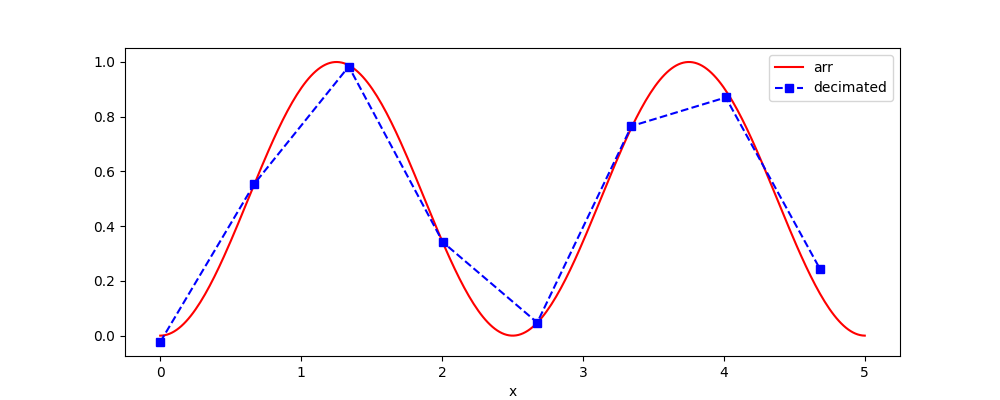
Our decimate() takes an xarray object
(possibly high dimensional) and a dimension name (if not 1D)
along which the signal should be decimated.
In [4]: arr_decimated = dsp.decimate(arr, q=20)

In [5]: arr_decimated
Out[5]:
<xarray.DataArray 'decimated' (x: 15)> Size: 120B
array([-0.00753439,  0.54815074,  0.9779414 ,  0.34671312,  0.03444491,
        0.77630424,  0.86853695,  0.16785983,  0.15635763,  0.9264748 ,
        0.7097045 ,  0.01718836,  0.42374382,  0.8500542 ,  0.7928993 ])
Coordinates:
  * x        (x) float64 120B 0.0 0.8406 1.681 2.522 ... 9.246 10.09 10.93 11.77
An alternative parameter to q is target_fs which is the new target sampling frequency to obtain, q = np.rint(current_fs / target_fs).
The return type is also a DataArray with coordinates.
In [6]: arr.plot(label='arr', color='r')
Out[6]: [<matplotlib.lines.Line2D at 0x7c56b30cdd10>]

In [7]: arr_decimated.plot.line('s--', label='decimated', color='b')
Out[7]: [<matplotlib.lines.Line2D at 0x7c56b30ce350>]

In [8]: plt.legend()
Out[8]: <matplotlib.legend.Legend at 0x7c56b461aba0>

In [9]: plt.show()
Savitzky-Golay LSQ filtering
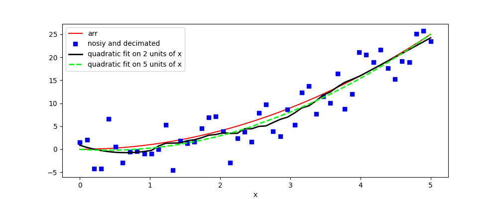
The Savitzky-Golay filter as a special type of a FIR filter which is equivalent to replacing filtered values by least-square fits of polynomials (or their derivatives) of a given order within a rolling window. For details see their Wikipedia page Such a filter is very useful when temporal or spatial features in the signal are of greater interest than frequency or wavenumber bands, respectively.
To demonstrate basic functionality of savgol_filter(), let’s create a simple example DataArray of the quadratic shape and add some noise:
In [10]: arr = xr.DataArray(np.linspace(0, 5, 50) ** 2,
   ....:                    dims=('x'), coords={'x': np.linspace(0, 5, 50)})
   ....:

In [11]: noise = np.random.normal(0,3,50)

In [12]: arr_noisy = arr + noise

In [13]: arr
Out[13]:
<xarray.DataArray (x: 50)> Size: 400B
array([0.00000000e+00, 1.04123282e-02, 4.16493128e-02, 9.37109538e-02,
       1.66597251e-01, 2.60308205e-01, 3.74843815e-01, 5.10204082e-01,
       6.66389005e-01, 8.43398584e-01, 1.04123282e+00, 1.25989171e+00,
       1.49937526e+00, 1.75968347e+00, 2.04081633e+00, 2.34277384e+00,
       2.66555602e+00, 3.00916285e+00, 3.37359434e+00, 3.75885048e+00,
       4.16493128e+00, 4.59183673e+00, 5.03956685e+00, 5.50812162e+00,
       5.99750104e+00, 6.50770512e+00, 7.03873386e+00, 7.59058726e+00,
       8.16326531e+00, 8.75676801e+00, 9.37109538e+00, 1.00062474e+01,
       1.06622241e+01, 1.13390254e+01, 1.20366514e+01, 1.27551020e+01,
       1.34943773e+01, 1.42544773e+01, 1.50354019e+01, 1.58371512e+01,
       1.66597251e+01, 1.75031237e+01, 1.83673469e+01, 1.92523948e+01,
       2.01582674e+01, 2.10849646e+01, 2.20324865e+01, 2.30008330e+01,
       2.39900042e+01, 2.50000000e+01])
Coordinates:
  * x        (x) float64 400B 0.0 0.102 0.2041 0.3061 ... 4.694 4.796 4.898 5.0
Our savgol_filter() takes an xarray object
(possibly high dimensional) and a dimension name (if not 1D)
along which the signal should be filtered.
The window length is given in the units of the dimension coordinates.
In [14]: arr_savgol2 = dsp.savgol_filter(arr_noisy, 0.5, 2)

In [15]: arr_savgol5 = dsp.savgol_filter(arr_noisy, 1.0, 2)

In [16]: arr_savgol2
Out[16]:
<xarray.DataArray 'savgol_filtered' (x: 50)> Size: 400B
array([-2.52956953e+00, -4.15762235e+00, -4.20598612e+00, -2.66963719e+00,
       -2.04449819e-01, -1.94955461e-02, -4.62698092e-01, -2.42289453e+00,
       -1.77771260e+00,  1.88485562e-01,  2.82140228e+00,  6.98884434e-01,
        2.08384764e+00,  2.21584535e+00,  3.15491298e+00,  2.30813298e+00,
        4.91977966e+00,  6.50566155e+00,  4.82235173e+00,  2.44942171e+00,
        2.87692176e+00,  4.03751403e+00,  4.92667167e+00,  5.92227490e+00,
        6.57591012e+00,  7.28526806e+00,  7.93406113e+00,  9.48760895e+00,
        8.06514621e+00,  9.39985253e+00,  9.20493682e+00,  1.17286719e+01,
        1.12085797e+01,  1.28627204e+01,  1.24821459e+01,  1.16588920e+01,
        1.01231024e+01,  1.38683848e+01,  1.77072327e+01,  1.72432754e+01,
        1.68834896e+01,  1.54980677e+01,  1.77989803e+01,  1.96170505e+01,
        2.08543326e+01,  1.88965300e+01,  2.34292894e+01,  2.61622879e+01,
        2.81953000e+01,  2.88327636e+01])
Coordinates:
  * x        (x) float64 400B 0.0 0.102 0.2041 0.3061 ... 4.694 4.796 4.898 5.0

In [17]: arr_savgol5
Out[17]:
<xarray.DataArray 'savgol_filtered' (x: 50)> Size: 400B
array([-3.37139966e+00, -3.09729165e+00, -2.78387593e+00, -2.43115251e+00,
       -2.03912140e+00, -1.60778258e+00, -1.09307979e+00, -1.56811955e-01,
       -5.65380288e-01,  2.38018347e-02,  6.20946953e-01,  1.31975776e+00,
        1.85741614e+00,  2.70337121e+00,  3.32128639e+00,  3.82053289e+00,
        4.03719895e+00,  4.52691936e+00,  3.77577715e+00,  4.27111274e+00,
        4.18847595e+00,  3.96285685e+00,  4.52683166e+00,  5.30839285e+00,
        7.02166747e+00,  7.21426526e+00,  7.87216100e+00,  8.44626327e+00,
        8.87959330e+00,  9.42781371e+00,  1.04008671e+01,  1.09071321e+01,
        1.14930297e+01,  1.10763651e+01,  1.18763454e+01,  1.26087357e+01,
        1.31590211e+01,  1.43470860e+01,  1.48056754e+01,  1.54941520e+01,
        1.73907007e+01,  1.79515301e+01,  1.75051232e+01,  1.85958526e+01,
        1.97631617e+01,  2.12206194e+01,  2.29495284e+01,  2.49498887e+01,
        2.72217004e+01,  2.97649635e+01])
Coordinates:
  * x        (x) float64 400B 0.0 0.102 0.2041 0.3061 ... 4.694 4.796 4.898 5.0
The return type is also a DataArray with coordinates.
In [18]: arr.plot(label='arr', color='r')
Out[18]: [<matplotlib.lines.Line2D at 0x7c56b30bf250>]

In [19]: arr_noisy.plot.line('s', label='noisy', color='b')
Out[19]: [<matplotlib.lines.Line2D at 0x7c56b30bf390>]

In [20]: arr_savgol2.plot(label='quadratic fit on 1 unit of x', color='k', linewidth=2)
Out[20]: [<matplotlib.lines.Line2D at 0x7c56b30bf4d0>]

In [21]: arr_savgol5.plot.line('--',label='quadratic fit on 2 units of x', linewidth=2, color='lime')
Out[21]: [<matplotlib.lines.Line2D at 0x7c56b30bfd90>]

In [22]: plt.legend()
Out[22]: <matplotlib.legend.Legend at 0x7c56b30bfed0>

In [23]: plt.show()
The other options (polynomial and derivative order) are the same as for scipy.signal.savgol_filter(), see savgol_filter() for details.
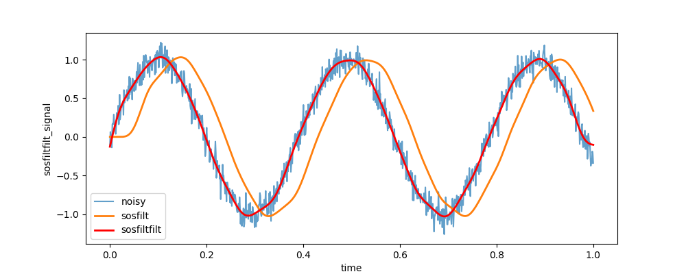
Second-order sections (SOS) filtering
The sosfilt() function provides a wrapper for scipy.signal.sosfilt() that applies a digital IIR filter in second-order sections format. This format is designed to minimize numerical precision errors for high-order filters by cascading second-order filter sections. The filter is defined by an array of second-order filter coefficients in the form (n_sections, 6), where each row corresponds to a second-order section with the first three columns providing the numerator coefficients and the last three providing the denominator coefficients.
For convenience, SOS filters can be easily created using scipy.signal.butter(), scipy.signal.cheby1(), scipy.signal.cheby2(), scipy.signal.ellip(), or scipy.signal.bessel() with output='sos'.
To demonstrate basic functionality of sosfilt() and sosfiltfilt(), let’s create a simple example with a 4th-order Butterworth low-pass filter:
In [24]: t = np.linspace(0, 1, 1000)

In [25]: sig = xr.DataArray(np.sin(16*t) + np.random.normal(0, 0.1, t.size),
   ....:                    coords=[('time', t)], name='signal')
   ....:

In [26]: from scipy.signal import butter

# Create a 8th-order Butterworth low-pass filter with cuttoff 20Hz
In [27]: sos = butter(8, 20, btype='low', fs=1/np.mean(np.diff(t)), output='sos')

# Apply the SOS filter along the 'time' dimension
In [28]: filtered = dsp.sosfilt(sos, sig, dim='time')

# Apply the zero-phase SOS filter along the 'time' dimension
In [29]: filtered_zero_phase = dsp.sosfiltfilt(sos, sig, dim='time')

In [30]: sig.plot(label='noisy', alpha=0.7)
Out[30]: [<matplotlib.lines.Line2D at 0x7c569b884910>]

In [31]: filtered.plot(label='sosfilt', linewidth=2)
Out[31]: [<matplotlib.lines.Line2D at 0x7c569b8851d0>]

In [32]: filtered_zero_phase.plot(label='sosfiltfilt', linewidth=2, color="red")
Out[32]: [<matplotlib.lines.Line2D at 0x7c569b885f90>]

In [33]: plt.legend()
Out[33]: <matplotlib.legend.Legend at 0x7c569b885090>

In [34]: plt.show()