Fourier Transform
xr-scipy wraps numpy.fft, for more convenient data analysis with
xarray.
Let us consider an example DataArray
In [1]: arr = xr.DataArray(np.sin(np.linspace(0, 15.7, 30)) ** 2,
   ...:                    dims=('x'), coords={'x': np.linspace(0, 5, 30)})
   ...:

In [2]: arr
Out[2]:
<xarray.DataArray (x: 30)> Size: 240B
array([0.00000000e+00, 2.65553207e-01, 7.80138804e-01, 9.97157371e-01,
       6.86089001e-01, 1.77354508e-01, 1.13381944e-02, 3.64384719e-01,
       8.61483534e-01, 9.74609903e-01, 5.83599545e-01, 1.03788678e-01,
       4.48385590e-02, 4.69366760e-01, 9.26433982e-01, 9.30537558e-01,
       4.77318618e-01, 4.81921327e-02, 9.89817591e-02, 5.75738105e-01,
       9.72044464e-01, 8.66939139e-01, 3.72066354e-01, 1.30863288e-02,
       1.71312250e-01, 6.78674515e-01, 9.96246419e-01, 7.86699011e-01,
       2.72616236e-01, 6.34122960e-05])
Coordinates:
  * x        (x) float64 240B 0.0 0.1724 0.3448 0.5172 ... 4.483 4.655 4.828 5.0
Our fft() takes an xarray object
(possibly high dimensional) and a coordinate name along which we compute
the Fourier transform.
In [3]: fft = xrscipy.fft.fft(arr, 'x')

In [4]: fft
Out[4]:
<xarray.DataArray (x: 30)> Size: 480B
array([ 1.45066531e+01-0.j        , -5.08969487e-01-0.05277866j,
       -5.64134191e-01-0.11825163j, -6.97777394e-01-0.22340666j,
       -1.09493558e+00-0.47978099j, -6.34538952e+00-3.59910605j,
        1.08016447e+00+0.76901603j,  4.01404487e-01+0.35285112j,
        2.07930614e-01+0.22420945j,  1.19289778e-01+0.15804858j,
        7.02940829e-02+0.11554961j,  4.06345993e-02+0.08441817j,
        2.20354770e-02+0.05946099j,  1.05946593e-02+0.03803481j,
        4.35028404e-03+0.01857428j,  2.36237341e-03-0.j        ,
        4.35028404e-03-0.01857428j,  1.05946593e-02-0.03803481j,
        2.20354770e-02-0.05946099j,  4.06345993e-02-0.08441817j,
        7.02940829e-02-0.11554961j,  1.19289778e-01-0.15804858j,
        2.07930614e-01-0.22420945j,  4.01404487e-01-0.35285112j,
        1.08016447e+00-0.76901603j, -6.34538952e+00+3.59910605j,
       -1.09493558e+00+0.47978099j, -6.97777394e-01+0.22340666j,
       -5.64134191e-01+0.11825163j, -5.08969487e-01+0.05277866j])
Coordinates:
  * x        (x) float64 240B 0.0 0.1933 0.3867 0.58 ... -0.58 -0.3867 -0.1933
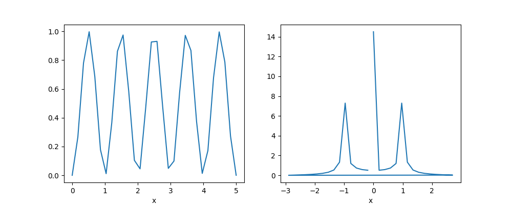
The coordinate x is also converted to frequency.
In [5]: plt.figure(figsize=(10, 4))
Out[5]: <Figure size 1000x400 with 0 Axes>

In [6]: plt.subplot(1, 2, 1)
Out[6]: <Axes: >

In [7]: arr.plot()
Out[7]: [<matplotlib.lines.Line2D at 0x7c56b3201a90>]

In [8]: plt.subplot(1, 2, 2)
Out[8]: <Axes: >

In [9]: np.abs(fft).plot()
Out[9]: [<matplotlib.lines.Line2D at 0x7c56b3215950>]

In [10]: plt.show()
Note
The coordinate values must be evenly spaced for FFT.
Multidimensional Fourier transform
xr-scipy also wraps the multidimensional Fourier transform,
such as rfftn()
Their usage is very similar to the above, where we just need to specify coordinates.
In [11]: arr = xr.DataArray(np.random.randn(30, 20) ** 2,
   ....:                    dims=('x', 'y'),
   ....:                    coords={'x': np.linspace(0, 5, 30),
   ....:                            'y': np.linspace(0, 5, 20)})
   ....:

In [12]: fftn = xrscipy.fft.fftn(arr, 'x', 'y')

In [13]: fftn
Out[13]:
<xarray.DataArray (x: 30, y: 20)> Size: 10kB
array([[ 6.80147367e+02-0.00000000e+00j, -5.40888999e+01-1.48914052e+01j,
         2.24071878e+01-6.83472672e+00j, -1.05248506e+01-1.98086495e+01j,
         3.30186673e+01+2.47699470e+01j, -4.10255035e+01+1.25478518e+01j,
         2.07742440e+01-2.10698675e+01j,  1.12280731e+01+8.16514918e+00j,
        -6.15766306e+01+1.53389009e+01j,  1.68000520e+01+3.08873987e+01j,
         6.91096924e+01-0.00000000e+00j,  1.68000520e+01-3.08873987e+01j,
        -6.15766306e+01-1.53389009e+01j,  1.12280731e+01-8.16514918e+00j,
         2.07742440e+01+2.10698675e+01j, -4.10255035e+01-1.25478518e+01j,
         3.30186673e+01-2.47699470e+01j, -1.05248506e+01+1.98086495e+01j,
         2.24071878e+01+6.83472672e+00j, -5.40888999e+01+1.48914052e+01j],
       [-9.78304942e+00-2.00060691e+01j, -3.01214418e+01-6.86851691e-01j,
         3.65704485e+01+2.64031486e+01j, -1.65402379e+01+5.18006959e+00j,
         5.75308280e+00+2.73910712e+01j, -2.48612360e+01-1.19071034e+01j,
        -1.90295095e+01+5.25959400e+01j, -7.66929151e+00-4.16255367e+00j,
        -3.41801537e+01+4.29905149e+01j,  1.23190320e+01+1.63252604e+01j,
        -4.84907294e+01-4.16601947e+01j,  1.07657876e+01-1.41656999e+01j,
        -3.39807068e+01+9.65027977e+00j,  5.89818080e+01-1.58963695e+00j,
        -2.24569277e+01+4.78807494e+00j,  2.29408613e+00-2.10730557e+01j,
         1.20560230e+00+2.45535230e+01j, -2.64074189e+01-1.52314832e+01j,
        -3.75456761e+00+6.28466305e+01j,  1.28963968e+01-3.01513717e+01j],
...
       [ 1.18390109e+01-1.69615481e+01j,  2.23641363e+01+2.98647685e-02j,
         8.93965329e+00-1.28033963e+01j, -6.17481319e+00-1.43282178e+01j,
         5.18844566e+01+3.92437600e+01j,  1.49904457e+01-1.62863784e+00j,
        -3.63069591e+01-2.63605337e+01j,  2.27092738e+01-1.09230345e+01j,
        -5.77461281e+00+2.23819916e+01j,  4.48110583e+01-2.09499730e+00j,
        -2.91364141e+01+4.57237154e+01j,  2.60820207e+01+1.08850196e+01j,
        -2.41167969e+01-8.25647322e+00j,  6.89571773e+00+7.65203935e+00j,
         1.99909029e+01+2.37322857e+01j, -7.38998869e+00-5.92937093e+00j,
        -3.26843493e+01-2.78910788e+01j,  1.51573868e+01-8.87107641e-02j,
         3.48168720e+00-3.93232365e+01j, -1.03891185e+01-3.07147965e+01j],
       [-9.78304942e+00+2.00060691e+01j,  1.28963968e+01+3.01513717e+01j,
        -3.75456761e+00-6.28466305e+01j, -2.64074189e+01+1.52314832e+01j,
         1.20560230e+00-2.45535230e+01j,  2.29408613e+00+2.10730557e+01j,
        -2.24569277e+01-4.78807494e+00j,  5.89818080e+01+1.58963695e+00j,
        -3.39807068e+01-9.65027977e+00j,  1.07657876e+01+1.41656999e+01j,
        -4.84907294e+01+4.16601947e+01j,  1.23190320e+01-1.63252604e+01j,
        -3.41801537e+01-4.29905149e+01j, -7.66929151e+00+4.16255367e+00j,
        -1.90295095e+01-5.25959400e+01j, -2.48612360e+01+1.19071034e+01j,
         5.75308280e+00-2.73910712e+01j, -1.65402379e+01-5.18006959e+00j,
         3.65704485e+01-2.64031486e+01j, -3.01214418e+01+6.86851691e-01j]])
Coordinates:
  * x        (x) float64 240B 0.0 0.1933 0.3867 0.58 ... -0.58 -0.3867 -0.1933
  * y        (y) float64 160B 0.0 0.19 0.38 0.57 ... -0.76 -0.57 -0.38 -0.19
In [14]: plt.figure(figsize=(10, 4))
Out[14]: <Figure size 1000x400 with 0 Axes>

In [15]: plt.subplot(1, 2, 1)
Out[15]: <Axes: >

In [16]: arr.plot()
Out[16]: <matplotlib.collections.QuadMesh at 0x7c56b320d6a0>

In [17]: plt.subplot(1, 2, 2)
Out[17]: <Axes: >

In [18]: np.abs(fftn.sortby('x').sortby('y')).plot()
Out[18]: <matplotlib.collections.QuadMesh at 0x7c56b32dbb10>

In [19]: plt.show()
