Spectral (FFT) analysis
xr-scipy wraps some of scipy spectral analysis functions such as scipy.signal.spectrogram(), scipy.signal.csd() etc. For convenience, the xrscipy.signal namespace will be imported under the alias dsp
In [1]: import xrscipy.signal as dsp
To demonstrate the basic functionality, let’s create two simple example DataArray at a similar frequency but one with a frequency drift and some noise:
In [2]: time_ax = np.arange(0,100,0.01)

In [3]: sig_1 = xr.DataArray(np.sin(100 * time_ax) + np.random.rand(len(time_ax))*3,
   ...:                      coords=[("time", time_ax)], name='sig_1')
   ...:

In [4]: sig_2 = xr.DataArray((np.cos(100 * time_ax) + np.random.rand(len(time_ax))*3 +
   ...:                       3*np.sin(30 * time_ax**1.3)),
   ...:                      coords=[("time", time_ax)], name='sig_2')
   ...:
Power spectra
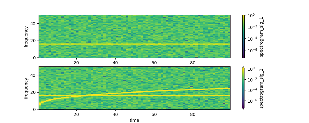
The spectrogram() function can be used directly on an xarray
DataArray object. The returned object is again an xarray.DataArray object.
In [5]: spec_1 = dsp.spectrogram(sig_1)

In [6]: spec_2 = dsp.spectrogram(sig_2)

In [7]: spec_2
Out[7]:
<xarray.DataArray 'spectrogram_sig_2' (frequency: 129, time: 77)> Size: 79kB
array([[2.44424801e-05, 5.22947169e-03, 2.89224670e-04, ...,
        1.49873467e-03, 7.65608700e-04, 9.59582636e-05],
       [1.75153585e-02, 1.89154990e-02, 7.80560915e-03, ...,
        1.44778153e-03, 1.09230319e-02, 9.86477734e-03],
       [2.67981444e-02, 1.72320528e-03, 1.77923215e-02, ...,
        3.47197400e-03, 7.94489056e-05, 1.24722011e-02],
       ...,
       [7.31455285e-03, 1.98518741e-02, 5.07390687e-03, ...,
        6.44165409e-03, 5.43732551e-03, 7.00189408e-03],
       [3.07786421e-03, 1.69232295e-03, 1.04356585e-03, ...,
        2.04653030e-02, 5.20056837e-04, 1.61887611e-02],
       [2.69532456e-03, 1.81679619e-05, 2.76618829e-03, ...,
        5.93410480e-03, 6.43149358e-03, 1.45961774e-02]], shape=(129, 77))
Coordinates:
  * time       (time) float64 616B 1.28 2.56 3.84 5.12 ... 96.0 97.28 98.56
  * frequency  (frequency) float64 1kB 0.0 0.3906 0.7812 ... 49.22 49.61 50.0
The frequency dimension coords are based on the transformed dimension (time in this case) coords sampling (i.e. inverse units). When the signal is 1D, the dimension does not have to be provided.
In [8]: norm = plt.matplotlib.colors.LogNorm()

In [9]: plt.subplot(211)
Out[9]: <Axes: >

In [10]: spec_1.plot(norm=norm)
Out[10]: <matplotlib.collections.QuadMesh at 0x755bcab49950>

In [11]: plt.subplot(212)
Out[11]: <Axes: >

In [12]: spec_2.plot(norm=norm)
Out[12]: <matplotlib.collections.QuadMesh at 0x755baf33dd10>

In [13]: plt.show()
These routines calculate the FFT on segments of the signal of a length controlled by nperseg and nfft parameters. The routines here offer a convenience parameter seglen which makes it possible to specify the segment length in the units of the transformed dimension’s coords. If seglen is specified, nperseg is then calculated from it and nfft is set using scipy.fftpack.next_fast_len (or to closest higher power of 2). A desired frequency resolution spacing df can be achieved by specifying seglen=1/df.
Another convenience parameter is overlap_ratio which calculates the noverlap parameter (by how many points the segments overlap) as noverlap = np.rint(overlap_ratio * nperseg)
For example, these parameters calculate the spectrogram with a higher frequency resolution and try to make for the longer segments by overlapping them by 75%.
In [14]: dsp.spectrogram(sig_1, seglen=1, overlap_ratio=0.75)
Out[14]:
<xarray.DataArray 'spectrogram_sig_1' (frequency: 51, time: 397)> Size: 162kB
array([[3.99319244e-04, 5.72385049e-06, 4.63213189e-04, ...,
        1.30700319e-03, 8.42935876e-04, 2.13630973e-03],
       [2.36519351e-03, 2.63675999e-03, 2.70759396e-03, ...,
        1.35248503e-02, 1.52467384e-02, 1.52477065e-02],
       [1.14508286e-03, 6.57120911e-03, 1.59951326e-02, ...,
        2.59556948e-02, 2.86589719e-02, 2.80344654e-02],
       ...,
       [3.22485304e-02, 5.98876777e-03, 4.75008719e-03, ...,
        1.27105913e-02, 1.10435949e-02, 2.60625766e-03],
       [6.48727646e-03, 4.24654407e-03, 5.71875070e-03, ...,
        3.54197551e-03, 4.97810155e-02, 5.84757962e-02],
       [7.82088430e-04, 3.02992866e-04, 8.29188527e-03, ...,
        1.46543043e-02, 4.78417261e-02, 3.80860346e-02]], shape=(51, 397))
Coordinates:
  * time       (time) float64 3kB 0.5 0.75 1.0 1.25 ... 98.75 99.0 99.25 99.5
  * frequency  (frequency) float64 408B 0.0 1.0 2.0 3.0 ... 47.0 48.0 49.0 50.0
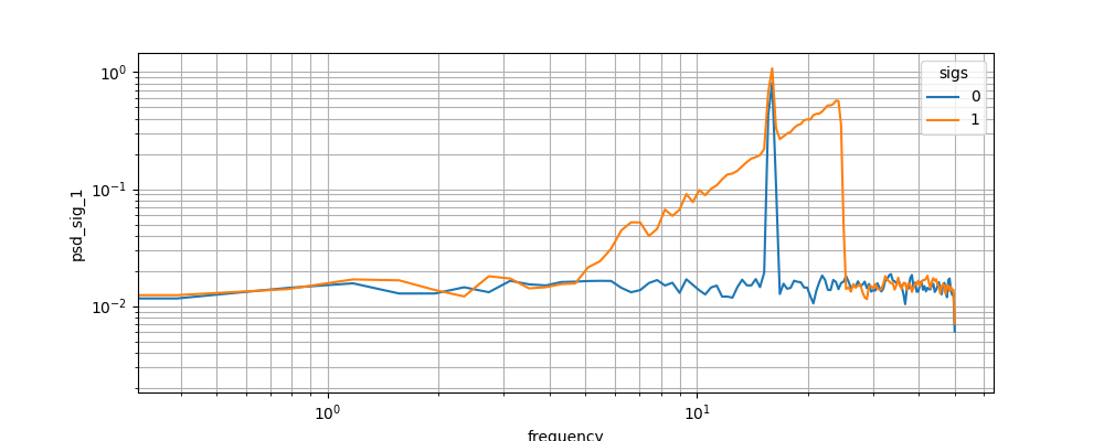
All the functions can be calculated on N-dimensional signals if the dimension is provided. Here the power spectral density (PSD) \(P_{xx}\) is calculated using Welch’s method (i.e. time average of the spectrogram) is shown
In [15]: sig_2D = xr.concat([sig_1,sig_2], dim="sigs")

In [16]: psd_2D = dsp.welch(sig_2D, dim="time")
In [17]: psd_2D.plot.line(x='frequency')
Out[17]:
[<matplotlib.lines.Line2D at 0x755baf31bed0>,
 <matplotlib.lines.Line2D at 0x755baf31bd90>]

In [18]: plt.loglog()
Out[18]: []

In [19]: plt.grid(which='both')

In [20]: plt.show()
Coherence
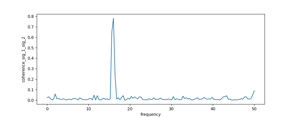
The same windowed FFT approach is also used to calculate the cross-spectral density \(P_{xy}\) (using xrscipy.signal.csd()) and from it coherency \(\gamma\) as
where \(\langle \dots \rangle\) is an average over the FFT windows, i.e. ergodicity is assumed.
In [21]: coh = dsp.coherence(sig_1, sig_2)

In [22]: coh[:10]
Out[22]:
<xarray.DataArray 'coherence_sig_1_sig_2' (frequency: 10)> Size: 80B
array([0.02385739, 0.03050104, 0.0140016 , 0.00035877, 0.0097276 ,
       0.05821104, 0.01216585, 0.01771338, 0.00619051, 0.00612246])
Coordinates:
  * frequency  (frequency) float64 80B 0.0 0.3906 0.7812 ... 2.734 3.125 3.516

In [23]: coh.plot()
Out[23]: [<matplotlib.lines.Line2D at 0x755baf1b0190>]

In [24]: plt.show()