Digital filters
xr-scipy wraps SciPy functions for digital signal processing. Wrappers for convenient functions such as scipy.signal.decimate() and scipy.signal.savgol_filter() are provided.
For convenience, the xrscipy.signal namespace will be imported under the alias dsp:
In [1]: import xrscipy.signal as dsp
Decimation
To demonstrate basic functionality of decimate(), let’s create a simple example DataArray:
In [2]: arr = xr.DataArray(np.sin(np.linspace(0, np.pi * 4, 300)) ** 2,
   ...:                    dims=('x'), coords={'x': np.linspace(0, np.pi * 4, 300)})
   ...:

In [3]: arr
Out[3]:
<xarray.DataArray (x: 300)> Size: 2kB
array([0.00000000e+00, 1.76531264e-03, 7.04878524e-03, 1.58131099e-02,
       2.79963995e-02, 4.35126247e-02, 6.22522218e-02, 8.40828655e-02,
       1.08850404e-01, 1.36379949e-01, 1.66477105e-01, 1.98929350e-01,
       2.33507531e-01, 2.69967481e-01, 3.08051749e-01, 3.47491411e-01,
       3.88007975e-01, 4.29315343e-01, 4.71121833e-01, 5.13132238e-01,
       5.55049914e-01, 5.96578868e-01, 6.37425855e-01, 6.77302444e-01,
       7.15927055e-01, 7.53026951e-01, 7.88340161e-01, 8.21617329e-01,
       8.52623476e-01, 8.81139660e-01, 9.06964522e-01, 9.29915705e-01,
       9.49831146e-01, 9.66570216e-01, 9.80014717e-01, 9.90069714e-01,
       9.96664206e-01, 9.99751627e-01, 9.99310177e-01, 9.95342973e-01,
       9.87878028e-01, 9.76968054e-01, 9.62690089e-01, 9.45144953e-01,
       9.24456537e-01, 9.00770928e-01, 8.74255374e-01, 8.45097109e-01,
       8.13502028e-01, 7.79693230e-01, 7.43909448e-01, 7.06403360e-01,
       6.67439806e-01, 6.27293918e-01, 5.86249176e-01, 5.44595406e-01,
       5.02626738e-01, 4.60639521e-01, 4.18930238e-01, 3.77793410e-01,
       3.37519512e-01, 2.98392931e-01, 2.60689947e-01, 2.24676791e-01,
       1.90607762e-01, 1.58723428e-01, 1.29248934e-01, 1.02392407e-01,
       7.83434858e-02, 5.72719872e-02, 3.93267020e-02, 2.46343464e-02,
       1.32986667e-02, 5.39970718e-03, 9.93244203e-04, 1.10392962e-04,
       2.75738749e-03, 8.91553669e-03, 1.85413563e-02, 3.15668761e-02,
...
       3.15668761e-02, 1.85413563e-02, 8.91553669e-03, 2.75738749e-03,
       1.10392962e-04, 9.93244203e-04, 5.39970718e-03, 1.32986667e-02,
       2.46343464e-02, 3.93267020e-02, 5.72719872e-02, 7.83434858e-02,
       1.02392407e-01, 1.29248934e-01, 1.58723428e-01, 1.90607762e-01,
       2.24676791e-01, 2.60689947e-01, 2.98392931e-01, 3.37519512e-01,
       3.77793410e-01, 4.18930238e-01, 4.60639521e-01, 5.02626738e-01,
       5.44595406e-01, 5.86249176e-01, 6.27293918e-01, 6.67439806e-01,
       7.06403360e-01, 7.43909448e-01, 7.79693230e-01, 8.13502028e-01,
       8.45097109e-01, 8.74255374e-01, 9.00770928e-01, 9.24456537e-01,
       9.45144953e-01, 9.62690089e-01, 9.76968054e-01, 9.87878028e-01,
       9.95342973e-01, 9.99310177e-01, 9.99751627e-01, 9.96664206e-01,
       9.90069714e-01, 9.80014717e-01, 9.66570216e-01, 9.49831146e-01,
       9.29915705e-01, 9.06964522e-01, 8.81139660e-01, 8.52623476e-01,
       8.21617329e-01, 7.88340161e-01, 7.53026951e-01, 7.15927055e-01,
       6.77302444e-01, 6.37425855e-01, 5.96578868e-01, 5.55049914e-01,
       5.13132238e-01, 4.71121833e-01, 4.29315343e-01, 3.88007975e-01,
       3.47491411e-01, 3.08051749e-01, 2.69967481e-01, 2.33507531e-01,
       1.98929350e-01, 1.66477105e-01, 1.36379949e-01, 1.08850404e-01,
       8.40828655e-02, 6.22522218e-02, 4.35126247e-02, 2.79963995e-02,
       1.58131099e-02, 7.04878524e-03, 1.76531264e-03, 2.39961565e-31])
Coordinates:
  * x        (x) float64 2kB 0.0 0.04203 0.08406 0.1261 ... 12.48 12.52 12.57
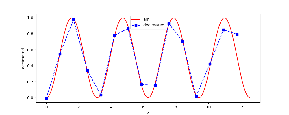
Our decimate() takes an xarray object
(possibly high dimensional) and a dimension name (if not 1D)
along which the signal should be decimated.
In [4]: arr_decimated = dsp.decimate(arr, q=20)

In [5]: arr_decimated
Out[5]:
<xarray.DataArray 'decimated' (x: 15)> Size: 120B
array([-0.00753439,  0.54815074,  0.9779414 ,  0.34671312,  0.03444491,
        0.77630424,  0.86853695,  0.16785983,  0.15635763,  0.9264748 ,
        0.7097045 ,  0.01718836,  0.42374382,  0.8500542 ,  0.7928993 ])
Coordinates:
  * x        (x) float64 120B 0.0 0.8406 1.681 2.522 ... 9.246 10.09 10.93 11.77
An alternative parameter to q is target_fs which is the new target sampling frequency to obtain, q = np.rint(current_fs / target_fs).
The return type is also a DataArray with coordinates.
In [6]: arr.plot(label='arr', color='r')
Out[6]: [<matplotlib.lines.Line2D at 0x72d7ff155810>]

In [7]: arr_decimated.plot.line('s--', label='decimated', color='b')
Out[7]: [<matplotlib.lines.Line2D at 0x72d7ff1556d0>]

In [8]: plt.legend()
Out[8]: <matplotlib.legend.Legend at 0x72d7ff54dd30>

In [9]: plt.show()
Savitzky-Golay LSQ filtering
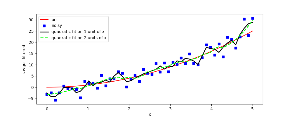
The Savitzky-Golay filter as a special type of a FIR filter which is equivalent to replacing filtered values by least-square fits of polynomials (or their derivatives) of a given order within a rolling window. For details see their Wikipedia page Such a filter is very useful when temporal or spatial features in the signal are of greater interest than frequency or wavenumber bands, respectively.
To demonstrate basic functionality of savgol_filter(), let’s create a simple example DataArray of the quadratic shape and add some noise:
In [10]: arr = xr.DataArray(np.linspace(0, 5, 50) ** 2,
   ....:                    dims=('x'), coords={'x': np.linspace(0, 5, 50)})
   ....:

In [11]: noise = np.random.normal(0,3,50)

In [12]: arr_noisy = arr + noise

In [13]: arr
Out[13]:
<xarray.DataArray (x: 50)> Size: 400B
array([0.00000000e+00, 1.04123282e-02, 4.16493128e-02, 9.37109538e-02,
       1.66597251e-01, 2.60308205e-01, 3.74843815e-01, 5.10204082e-01,
       6.66389005e-01, 8.43398584e-01, 1.04123282e+00, 1.25989171e+00,
       1.49937526e+00, 1.75968347e+00, 2.04081633e+00, 2.34277384e+00,
       2.66555602e+00, 3.00916285e+00, 3.37359434e+00, 3.75885048e+00,
       4.16493128e+00, 4.59183673e+00, 5.03956685e+00, 5.50812162e+00,
       5.99750104e+00, 6.50770512e+00, 7.03873386e+00, 7.59058726e+00,
       8.16326531e+00, 8.75676801e+00, 9.37109538e+00, 1.00062474e+01,
       1.06622241e+01, 1.13390254e+01, 1.20366514e+01, 1.27551020e+01,
       1.34943773e+01, 1.42544773e+01, 1.50354019e+01, 1.58371512e+01,
       1.66597251e+01, 1.75031237e+01, 1.83673469e+01, 1.92523948e+01,
       2.01582674e+01, 2.10849646e+01, 2.20324865e+01, 2.30008330e+01,
       2.39900042e+01, 2.50000000e+01])
Coordinates:
  * x        (x) float64 400B 0.0 0.102 0.2041 0.3061 ... 4.694 4.796 4.898 5.0
Our savgol_filter() takes an xarray object
(possibly high dimensional) and a dimension name (if not 1D)
along which the signal should be filtered.
The window length is given in the units of the dimension coordinates.
In [14]: arr_savgol2 = dsp.savgol_filter(arr_noisy, 0.5, 2)

In [15]: arr_savgol5 = dsp.savgol_filter(arr_noisy, 1.0, 2)

In [16]: arr_savgol2
Out[16]:
<xarray.DataArray 'savgol_filtered' (x: 50)> Size: 400B
array([-2.52956953e+00, -4.15762235e+00, -4.20598612e+00, -2.66963719e+00,
       -2.04449819e-01, -1.94955461e-02, -4.62698092e-01, -2.42289453e+00,
       -1.77771260e+00,  1.88485562e-01,  2.82140228e+00,  6.98884434e-01,
        2.08384764e+00,  2.21584535e+00,  3.15491298e+00,  2.30813298e+00,
        4.91977966e+00,  6.50566155e+00,  4.82235173e+00,  2.44942171e+00,
        2.87692176e+00,  4.03751403e+00,  4.92667167e+00,  5.92227490e+00,
        6.57591012e+00,  7.28526806e+00,  7.93406113e+00,  9.48760895e+00,
        8.06514621e+00,  9.39985253e+00,  9.20493682e+00,  1.17286719e+01,
        1.12085797e+01,  1.28627204e+01,  1.24821459e+01,  1.16588920e+01,
        1.01231024e+01,  1.38683848e+01,  1.77072327e+01,  1.72432754e+01,
        1.68834896e+01,  1.54980677e+01,  1.77989803e+01,  1.96170505e+01,
        2.08543326e+01,  1.88965300e+01,  2.34292894e+01,  2.61622879e+01,
        2.81953000e+01,  2.88327636e+01])
Coordinates:
  * x        (x) float64 400B 0.0 0.102 0.2041 0.3061 ... 4.694 4.796 4.898 5.0

In [17]: arr_savgol5
Out[17]:
<xarray.DataArray 'savgol_filtered' (x: 50)> Size: 400B
array([-3.37139966e+00, -3.09729165e+00, -2.78387593e+00, -2.43115251e+00,
       -2.03912140e+00, -1.60778258e+00, -1.09307979e+00, -1.56811955e-01,
       -5.65380288e-01,  2.38018347e-02,  6.20946953e-01,  1.31975776e+00,
        1.85741614e+00,  2.70337121e+00,  3.32128639e+00,  3.82053289e+00,
        4.03719895e+00,  4.52691936e+00,  3.77577715e+00,  4.27111274e+00,
        4.18847595e+00,  3.96285685e+00,  4.52683166e+00,  5.30839285e+00,
        7.02166747e+00,  7.21426526e+00,  7.87216100e+00,  8.44626327e+00,
        8.87959330e+00,  9.42781371e+00,  1.04008671e+01,  1.09071321e+01,
        1.14930297e+01,  1.10763651e+01,  1.18763454e+01,  1.26087357e+01,
        1.31590211e+01,  1.43470860e+01,  1.48056754e+01,  1.54941520e+01,
        1.73907007e+01,  1.79515301e+01,  1.75051232e+01,  1.85958526e+01,
        1.97631617e+01,  2.12206194e+01,  2.29495284e+01,  2.49498887e+01,
        2.72217004e+01,  2.97649635e+01])
Coordinates:
  * x        (x) float64 400B 0.0 0.102 0.2041 0.3061 ... 4.694 4.796 4.898 5.0
The return type is also a DataArray with coordinates.
In [18]: arr.plot(label='arr', color='r')
Out[18]: [<matplotlib.lines.Line2D at 0x72d7ff1420d0>]

In [19]: arr_noisy.plot.line('s', label='noisy', color='b')
Out[19]: [<matplotlib.lines.Line2D at 0x72d7ff142210>]

In [20]: arr_savgol2.plot(label='quadratic fit on 1 unit of x', color='k', linewidth=2)
Out[20]: [<matplotlib.lines.Line2D at 0x72d7ff142350>]

In [21]: arr_savgol5.plot.line('--',label='quadratic fit on 2 units of x', linewidth=2, color='lime')
Out[21]: [<matplotlib.lines.Line2D at 0x72d7ff142c10>]

In [22]: plt.legend()
Out[22]: <matplotlib.legend.Legend at 0x72d7ff143110>

In [23]: plt.show()
The other options (polynomial and derivative order) are the same as for scipy.signal.savgol_filter(), see savgol_filter() for details.